Radial Boundary Scan

Introduction

/	Measure→Perform Selected Scan
Keyboard	Main Menu	Toolbar

Radial Boundary Scan Setup Tool

The Radial Boundary Surface Scan Tool is designed to capture uniform row and column conforming data point clouds while probing in the –Z direction. The Scan Tool will “walk” the surface adjusting its Z probing height between data points allowing data clouds to be built on complex surfaces.

The Radial Boundary Surface Scan Tool behaves exactly like the Boundary Surface Scan Tool described in the previous section. The differences between the scan tools are the shape of the boundary. This scan tool has a circular boundary area.

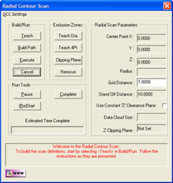
Step 1 - Defining the boundary of the scan area

To define the boundary, select <Teach>. You will be prompted to capture points along the perimeter of the scan area. When you have captured 3 or more data points, press the Terminate key, <F5>. The scan tool will calculate the diameter and position then populates the cells in the Radial Scan Parameters Group with the results.

Step 2 – Establishing the grid density

Ensure the Grid Distance value has the proper data point density value you want to scan. This Grid Distance is the distance between columns and rows.

Step 3 – Building the Motion Path

Build the initial motion map through the use of <Build Path>. The Scan Tool will report the total number of points that will be captured based on the current settings.

Adjustments can now be made to the motion path. These adjustments include changing the Grid Distance and the building of exclusion zones.

To change the point density, enter a new value in Grid Distance and press <Build Path> again. This will discard the existing motion path and compute a new one based on the changed Grid Distance value. NOTE: Making a change to the Grid Distance and then computing a new motion path will delete any existing exclusion zones.

To review how the scan tools create rows and columns, please read Understanding the Data Cloud Structure.

Step 4 – Exclusion Zones

One very important feature of the Scan Tool is the ability to eliminate areas within the defined scan boundaries. A common example might be a hole through the surface you are scanning. There are two types of Exclusion Zones available.

Diameter Exclusion Zone:

This tool works well to define exclusion zones around holes. Building a zone starts by pressing the <Teach Dia> button which prompts you to capture data points around the area to exclude.

When you have captured sufficient points, press the terminate key, <F5>. The scan tool will calculate the exclude area and determine the number of data points that will be excluded. Press <Remove> to complete the exclusion.

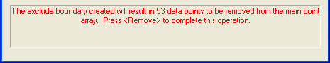Exclusion Zone Confirmation Message

4-Point Boundary Exclusion Zone:

This exclusion zone shape has the same characteristics as the boundary definitions in Step 1. To build the zone, press <Teach 4Pt> and then capture the 4 data points.

After the last point was captured, The scan tool will calculate the exclude area and determine the number of data points that will be excluded. Press <Remove> to complete the exclusion.

The surface may require several exclusion zones to be defined. You can create as many exclusion zones as necessary to build a proper scan.

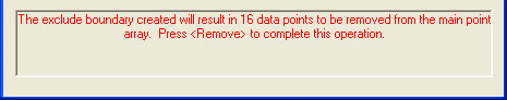Exclusion Zone Confirmation Message

Step 5 – Establish a Clipping Plane

If you require your scan boundary to extend beyond the surface, setting a Clipping Plane will help clear unwanted data points. Here we have an example of a scan that was done on a fan blade assembly. The boundary extended beyond the fan and included the surface plate the fan was positioned on.

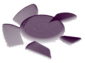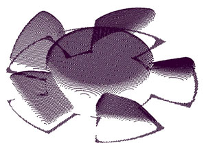Clipping Plane Active	Clipping Plane NOT Active

The added data points on the surface plate would interfere with spline operations and result in poor surface generation by CAD systems.

To establish a Clipping Plane, press <Clipping Plane>. You will then capture one data point on the surface that you want excluded from the final data cloud. During the scan process, each captured point will be evaluated and if it has a Z value equal to, or below, the Clipping Plane, if it does it will be discarded.

Step 6 – Use Z Clearance Height

The motion required to perform surface following by the scan tool involves the comparing the Z component of the current data point to the previous data:

Z_delta = Z_{current pt} – Z_{previous pt}

That difference is then added to the next data point to be scanned.

Z_{next pt} = Z_{current pt} + Z_delta

This is the simple explanation of contour following tool, there are other filters and controls in place to enhance the surface following capabilities.

The Z Clearance Height setting takes over the Z component adjustment formula and builds the motion path by using a constant Z height. Using the fan blade as an example, the step from the surface plate to the upper edge of the blade was over 1.25”. The CMM would approach this large step and crash.

Using the Z Clearance Height, you would set the height sufficient to clear the entire fan, then every data point would retract to that height before proceeding to the next data point assuring full clearance for all steps.

Step – 7 Stand Off and Over Travel

From the drop down menu, choose [DCC Settings→Standoff Distance]. The standoff distance should be sufficient to clear any vertical steps on the surface. Under [DCC Settings→Over Travel Distance], should be sufficient to drop off a vertical step and still locate the data point.

Step 8 – Execute

To begin the scanning operation, press <Execute>. The system will prompt you to position the CMM over the first data point in the motion path. When you have the CMM in that position, press the <IP> button on the joystick controller. Depending upon whether the Z Clearance Height is in effect will determine how the scan operation will take place.

Related Procedures:

Select Scan Method, 4-Point Boundary Scan, Line Scan, GeoTracer, Cardinal Splines, Export Tool