Helmel Engineering Products, Inc. Customer Support -- Tech Note #1
Curved Surface Measurement with Vector Point:
Applies to: Geomet 101 with GeoPlus, Geomet 301, Geomet 501.
Last updated:
Saturday January 15, 2011.
NOTICE
Information contained within this document is subject to change without notice. No part
of this document may be reproduced or transmitted in any form or by any means, electronic
or mechanical, for any purpose without written authorization from Helmel Engineering
Products, Inc.
This document contains proprietary subject matter of Helmel Engineering Products, Inc.
and its receipt or possession does not convey any rights to reproduce disclose its content
or to manufacture, use or sell anything it may describe. Reproduction, disclosure or use
without specific written authorization of Helmel Engineering Products, Inc. is strictly
forbidden.
© Helmel Engineering Products, Inc. 1985 - 2005. All right reserved.
GEOMET®, MICROSTAR® are trademarks of
Helmel Engineering Products, Inc.
Introduction
Technical Note #1 - Curved Surface Measurement with Vector Point
First Published January, 21, 1987
Dr. Jon M. Baldwin - Vice President Geomet Systems - a wholly owned division of Helmel
Engineering Products, Inc.
Edited October 14, 2003 - Edward R. Yaris - Software Development Manager, Helmel
Engineering Products, Inc.
Why Have Vector Point on Manual Coordinate Measuring Machines?
The answer to this question is simple and short. It provides a capability
for manual CMMs in an area normally considered to be the exclusive province
of computer controlled CMMs, namely the inspection of profiles on simple
(2D) and compound (3D) curved surfaces without the use of sharply pointed
probes. Granted, the measurement process involves iteratively homing in on a
target location and thus can be tedious, but it is no more so than
techniques that do use pointed probes with all their disadvantages and
dangers. A computer controlled CMM capable of driving accurately along a
specified vector to a specified target is obviously the instrument of choice
to solve this problem but is often not available or is too expensive to
justify for the occasional application; thus there has been interest in
providing this capability on manual CMMs.
Statement of the Problem
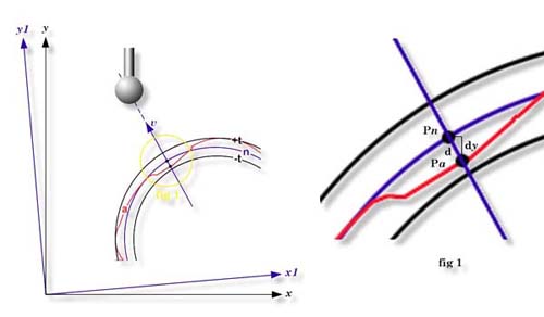
The nature of the problem to be solved is easily seen by reference to Figure 1, which,
for simplicity, shows a 2D example. The problem and its solution in 3D are identical,
being merely complicated by the need for a proper probe radius correction in space rather
than in the plane.
 |
| figure 1, Vector Point Problem |
Shown in the figure is a nominal surface, n, along with
the actual part surface, a, and allowed profile limits, +t
and –t. We wish to determine, at selected points, the deviation of
the actual surface from the nominal. Two pairs of axes, x and y,
of the machine coordinate system (MCS) and x1 and y1,
of the part coordinate system (PCS) are shown. Ideally, we would use a spherical probe and
approach the nominal point to be inspected, Pn, along the
nominal normal vector, v. Assuming the probe radius and errors
in the actual surface both are small compared to the radius of curvature at Pn,
the probe would contact the actual surface at point Pa, also
along the normal vector v, the probe center would also fall
along v and the probe radius correction and thus the deviation
of the actual surface from ideality could be simply computed. This is, in fact, what is
done when one makes this measurement with a computer controlled CMM having vector drive
capability.
We will note in passing that the inspection requirement may call for reporting either
the total deviation, d, along the normal vector or its
component, dy, parallel to the part coordinate system (PCS) axis
most nearly perpendicular to the surface. This has no effect on the measurement process,
but we will return to this matter later on. We will also note in passing that the first
assumption made above, namely that the probe radius is small compared to the radius of
curvature of the part surface, is not particular to the manual CMM problem but applies as
well to at least some curved surface measuring algorithms designed for use with motorized
vector drive CMMs.
If we try this same measurement with a manual CMM we find that since the CMM is not
easily moved along the specified normal vector with any degree of accuracy we have trouble
making even the point of contact with the nominal surface, never mind the point of contact
with the actual surface, fall as it should.
A Solution to the Problem – Normal Vector Point
The only axis along which we can accurately drive a manual CMM is one of the MCS axes,
so we will begin with that. Since we know the radius of the measuring probe it is easy to
calculate a two dimensional location in the MCS, to which we can drive the probe and,
having locked the CMM axes on this target, drive along the third CMM axis such that the
first point at which the probe contacts the nominal surface will be Pn.
 |
 |
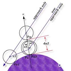
| figure 2, Approach Directions, Normal Vector
Point |
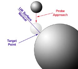
figure 3,
Manual CMM Approach |
Refer to Figure 2. We are not out of the woods yet. Even if we are
successful in arriving at the desired point Pn on the nominal
surface, we find that if the actual surface is not ideal we will miss Pa
and so will, in general, report an error greater than actually exist. To illustrate, let
us assume we have computed a target point on an MCS axis as indicated above. We will
generally want to move along the MCS axis most nearly perpendicular to the surface and it
does not really matter how far away from the part we begin. We simply lock two of the
machine axes and approach the part surface along the vector labeled "approach
axis", arriving at the nominal location of the surface with the probe center and the
nominal contact point, Pn, both lying on the nominal normal
vector, v. However, we have yet to contact the actual surface,
so we proceed further along the approach axis until contact is made at point Pa1.
Obviously, we have not ended up exactly where we would like to be. We were hoping to get
to point Pa and then the sought-for-error would have been simply
Pa-Pn, but we have missed. The error
is not anything we could have compensated for ahead of time since it is a function of the
actual surface location, a thing we were totally uninformed about until just this minute.
We now have some, rather limited, knowledge about the actual location of the surface and
can use that knowledge to refine our approach.
As a device to evaluate the extent to which we have accomplished the desired objective,
namely, to arrive at the actual surface with both the probe center and the contact point
on the normal vector, we will introduce the concept of the probing error. The probing
error will be defined as the normal distance from the ball center at contact and the
nominal normal vector, v, and is shown as e1
for the first probing in Figure 2. We would compare e1 to some
predetermined acceptable value which we will call the probing error limit, e.
(In the actual implementation of vector point, a value for e =(+t
+ 1 - t1)/5 is suggested but may be changed by the
user).
If e1 <= e then the attempt to measure the desired
target point is considered to have been successful and the measurement results are
printed.
If e1 > e the value of e1 is
displayed and the user is given the option to accept the results or to attempt further
refinement of the probing location. The new approach is generated by projecting the
current probe center location back onto the nominal normal vector, v,
to get a refined estimate of where we want the probe to be at the time it contacts the
actual surface. The machine axis vector passing through this new point becomes the new
approach axis, along which a new 2D target is calculated, and the process is repeated to
give a new point of contact, Pa2, and associated probing error, e2.
The process may be repeated indefinitely until either the probing error limit criterion is
satisfied or the user decides the disparity between the actual and nominal surfaces is so
large that the probing error limit will always be exceeded.
The final contact point, in this case Pa2, is projected onto
the normal vector, v, and the distance, da2,
along v from Pn to Pa2
is taken as the final estimate of the normal deviation of the surface from its ideal
location.
Paraxial Vector Point
The foregoing discussion was concerned with the situation wherein the deviation is to
be measured along the direction of the nominal normal to the surface at the target
location. This is referred to, naturally enough, as the normal deviation case. It is also
possible to encounter the situation where the deviation is to be taken in parallel to the PCS axis that is most
nearly perpendicular to the nominal surface. We will refer to this as the paraxial
deviation case. The computations are only slightly more complicated and are illustrated in
Figure 3.
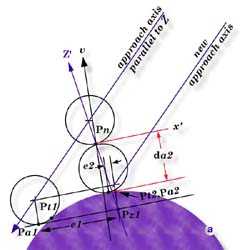 |
| figure 3, Paraxial Vector Point |
Once again, the nominal target point, Pn, is
defined in terms of its coordinates in the PCS and of the nominal normal vector, v,
to the surface at that point. The definition of the initial approach axis is identical to
the normal deviation case. The final objective is different. We now wish to have the probe
arrive at the actual surface such that the contact point, P, lies along a
vector, z’, that is parallel to the PCS axis most nearly
parallel to the nominal normal vector, v, and that passes
through Pa. Once again, since the surface is not ideal, the
probe actually makes contact at Pt1, a point we cannot locate
exactly but must estimate. We can do this by making an approximate correction for the
probe radius parallel to the nominal normal vector to get point Pa1.
We can calculate a probing error, e1, by first constructing a
plane tangent to the probe and passing through Pa1 then
intersecting that plane with z’ to get point Pz1.
The probing error e is the distance from Pa1 to Pz1.
Assuming that e1 > e and that the user elects to
refine the measurement, a new approach axis is constructed parallel to the first but
passing through the probe center location that corresponds to placing the probe surface at
Pz1. Approaching the actual surface along this (machine) axis
results in a contact at Pt2, and estimated contact at Paz and an
improved probing error, e2. If this probing error is judged small enough,
the paraxial deviation, da2, is reported parallel to z’.
Experimenting with Vector Point
Before you get too serious about using vector point in a real application,
it may be helpful to you to play with it a bit. One easy way to do this is
to use the reference sample files found in the Measured Point Knowledgebase
pages found at:
Knowledgebase→Measured
Features→Point→Method
5
There are several examples to follow to help in understanding the
application of Vector Points on DCC and manual style CMMs.
|